Metek MRR2

import cmweather  # noqa
import matplotlib.pyplot as plt
from open_radar_data import DATASETS

import xradar as xd

xd.io.open_metek_datatree supports the Metek MRR2 processed (.pro, .ave) and raw (.raw) files. The initalized datatree will contain all of the vertically pointing radar data in one sweep.

In this example, we are loading the 60 s average files from the MRR2 sampling a rain event over the Argonne Testbed for Multiscale Observational Science at Argonne National Laboratory in the Chicago suburbs.

mrr_test_file = DATASETS.fetch("0308.pro.gz")
!gunzip -f $mrr_test_file
with xd.io.open_metek_datatree(mrr_test_file[:-3]) as ds:
    display(ds)

Downloading file '0308.pro.gz' from 'https://github.com/openradar/open-radar-data/raw/main/data/0308.pro.gz' to '/home/docs/.cache/open-radar-data'.

<xarray.DatasetView> Size: 232B
Dimensions:              ()
Data variables:
    volume_number        int64 8B 0
    platform_type        <U5 20B 'fixed'
    instrument_type      <U5 20B 'radar'
    time_coverage_start  <U20 80B '2024-03-08T23:00:00Z'
    time_coverage_end    <U20 80B '2024-03-08T23:59:57Z'
    latitude             float64 8B ...
    longitude            float64 8B ...
    altitude             float64 8B ...
Attributes:
    Conventions:      None
    instrument_name:  None
    version:          None
    title:            None
    institution:      None
    references:       None
    source:           None
    history:          None
    comment:          im/exported using xradar

xarray.DataTree

• Groups: (4)
  <xarray.DatasetView> Size: 18MB
  Dimensions:                      (sample: 64, time: 362, range: 31, index: 11222)
  Coordinates:
      velocity_bins                (sample) float64 512B ...
    * range                        (range) float64 248B 150.0 300.0 ... 4.65e+03
    * time                         (time) datetime64[ns] 3kB 2024-03-08T23:00:0...
  Dimensions without coordinates: sample, index
  Data variables: (12/17)
      transfer_function            (time, range) float64 90kB ...
      spectral_reflectivity        (index, sample) float64 6MB ...
      drop_size                    (index, sample) float64 6MB ...
      drop_number_density          (index, sample) float64 6MB ...
      percentage_valid_spectra     (time) float64 3kB ...
      path_integrated_attenuation  (time, range) float64 90kB ...
      ...                           ...
      altitude                     float64 8B ...
      longitude                    float64 8B ...
      latitude                     float64 8B ...
      spectrum_index               (time, range) float64 90kB ...
      azimuth                      (time) float64 3kB ...
      elevation                    (time) float64 3kB ...

  sweep_0

  • Groups: (0)
  • Dimensions:
    • sample: 64
    • time: 362
    • range: 31
    • index: 11222
  • Coordinates: (3)
    • velocity_bins
      (sample)
      float64
      ...

      long_name :

      Doppler velocity bins

      standard_name :

      doppler_velocity_bins

      units :

      m s-1

      [64 values with dtype=float64]

    • range
      (range)
      float64
      150.0 300.0 ... 4.5e+03 4.65e+03

      long_name :

      Range from radar

      standard_name :

      range

      units :

      m

      array([ 150.,  300.,  450.,  600.,  750.,  900., 1050., 1200., 1350., 1500.,
             1650., 1800., 1950., 2100., 2250., 2400., 2550., 2700., 2850., 3000.,
             3150., 3300., 3450., 3600., 3750., 3900., 4050., 4200., 4350., 4500.,
             4650.])

    • time
      (time)
      datetime64[ns]
      2024-03-08T23:00:00 ... 2024-03-...

      standard_name :

      time

      units :

      seconds since 1970-01-01T00:00:00Z

      array(['2024-03-08T23:00:00.000000000', '2024-03-08T23:00:10.000000000',
             '2024-03-08T23:00:20.000000000', ..., '2024-03-08T23:59:37.000000000',
             '2024-03-08T23:59:47.000000000', '2024-03-08T23:59:57.000000000'],
            dtype='datetime64[ns]')

  • Data variables: (17)
    • transfer_function
      (time, range)
      float64
      ...

      long_name :

      Transfer function

      standard_name :

      transfer_function

      units :

      1

      [11222 values with dtype=float64]

    • spectral_reflectivity
      (index, sample)
      float64
      ...

      long_name :

      Spectral reflectivity

      standard_name :

      equivalent_reflectivity_factor

      units :

      dB

      [718208 values with dtype=float64]

    • drop_size
      (index, sample)
      float64
      ...

      long_name :

      Drop size

      standard_name :

      drop_size

      units :

      mm

      [718208 values with dtype=float64]

    • drop_number_density
      (index, sample)
      float64
      ...

      long_name :

      Raindrop number density

      standard_name :

      raindrop_number_density

      units :

      m-4

      [718208 values with dtype=float64]

    • percentage_valid_spectra
      (time)
      float64
      ...

      long_name :

      Percentage of spectra that are valid

      standard_name :

      percentage_valid_spectra

      units :

      percent

      [362 values with dtype=float64]

    • path_integrated_attenuation
      (time, range)
      float64
      ...

      long_name :

      Path integrated attenuation

      standard_name :

      path_integrated_attenuation

      units :

      dB

      [11222 values with dtype=float64]

    • corrected_reflectivity
      (time, range)
      float64
      ...

      long_name :

      Attenuation-corrected Radar reflectivity factor

      standard_name :

      equivalent_radar_reflectivity_factor

      units :

      dBZ

      [11222 values with dtype=float64]

    • reflectivity
      (time, range)
      float64
      ...

      long_name :

      Radar reflectivity factor

      standard_name :

      equivalent_radar_reflectivity_factor

      units :

      dBZ

      [11222 values with dtype=float64]

    • rainfall_rate
      (time, range)
      float64
      ...

      long_name :

      Rainfall rate

      standard_name :

      rainfall_rate

      units :

      mm hr-1

      [11222 values with dtype=float64]

    • liquid_water_content
      (time, range)
      float64
      ...

      long_name :

      Liquid water content

      standard_name :

      liquid_water_content

      units :

      g m-3

      [11222 values with dtype=float64]

    • velocity
      (time, range)
      float64
      ...

      long_name :

      Radial velocity of scatterers toward instrument

      standard_name :

      radial_velocity_of_scatterers_toward_instrument

      units :

      m s-1

      [11222 values with dtype=float64]

    • altitude
      ()
      float64
      ...

      long_name :

      altitude

      units :

      meters

      standard_name :

      altitude

      [1 values with dtype=float64]

    • longitude
      ()
      float64
      ...

      long_name :

      longitude

      units :

      degrees_east

      standard_name :

      longitude

      [1 values with dtype=float64]

    • latitude
      ()
      float64
      ...

      long_name :

      latitude

      units :

      degrees_north

      positive :

      up

      standard_name :

      latitude

      [1 values with dtype=float64]

    • spectrum_index
      (time, range)
      float64
      ...

      long_name :

      Spectrum index

      standard_name :

      spectrum_index

      units :

      1

      [11222 values with dtype=float64]

    • azimuth
      (time)
      float64
      ...

      standard_name :

      ray_azimuth_angle

      long_name :

      azimuth_angle_from_true_north

      units :

      degrees

      axis :

      radial_azimuth_coordinate

      [362 values with dtype=float64]

    • elevation
      (time)
      float64
      ...

      standard_name :

      ray_elevation_angle

      long_name :

      elevation_angle_from_horizontal_plane

      units :

      degrees

      axis :

      radial_elevation_coordinate

      [362 values with dtype=float64]

  • Attributes: (0)

  <xarray.DatasetView> Size: 0B
  Dimensions:  ()
  Data variables:
      *empty*

  radar_parameters

  • Groups: (0)
  • Dimensions:
  • Coordinates: (0)
  • Data variables: (0)
  • Attributes: (0)

  <xarray.DatasetView> Size: 0B
  Dimensions:  ()
  Data variables:
      *empty*

  georeferencing_correction

  • Groups: (0)
  • Dimensions:
  • Coordinates: (0)
  • Data variables: (0)
  • Attributes: (0)

  <xarray.DatasetView> Size: 0B
  Dimensions:  ()
  Data variables:
      *empty*

  radar_calibration

  • Groups: (0)
  • Dimensions:
  • Coordinates: (0)
  • Data variables: (0)
  • Attributes: (0)

• Dimensions:
• Coordinates: (0)
• Inherited coordinates: (0)
• Data variables: (8)
  • volume_number
    ()
    int64
    0

    array(0)

  • platform_type
    ()
    <U5
    'fixed'

    array('fixed', dtype='<U5')

  • instrument_type
    ()
    <U5
    'radar'

    array('radar', dtype='<U5')

  • time_coverage_start
    ()
    <U20
    '2024-03-08T23:00:00Z'

    array('2024-03-08T23:00:00Z', dtype='<U20')

  • time_coverage_end
    ()
    <U20
    '2024-03-08T23:59:57Z'

    array('2024-03-08T23:59:57Z', dtype='<U20')

  • latitude
    ()
    float64
    ...

    long_name :

    latitude

    units :

    degrees_north

    positive :

    up

    standard_name :

    latitude

    [1 values with dtype=float64]

  • longitude
    ()
    float64
    ...

    long_name :

    longitude

    units :

    degrees_east

    standard_name :

    longitude

    [1 values with dtype=float64]

  • altitude
    ()
    float64
    ...

    long_name :

    altitude

    units :

    meters

    standard_name :

    altitude

    [1 values with dtype=float64]

• Attributes: (9)

  Conventions :

  None

  instrument_name :

  None

  version :

  None

  title :

  None

  institution :

  None

  references :

  None

  source :

  None

  history :

  None

  comment :

  im/exported using xradar

View the structure of the loaded datatree.

ds["sweep_0"]

<xarray.DatasetView> Size: 18MB
Dimensions:                      (sample: 64, time: 362, range: 31, index: 11222)
Coordinates:
    velocity_bins                (sample) float64 512B ...
  * range                        (range) float64 248B 150.0 300.0 ... 4.65e+03
  * time                         (time) datetime64[ns] 3kB 2024-03-08T23:00:0...
Dimensions without coordinates: sample, index
Data variables: (12/17)
    transfer_function            (time, range) float64 90kB ...
    spectral_reflectivity        (index, sample) float64 6MB ...
    drop_size                    (index, sample) float64 6MB ...
    drop_number_density          (index, sample) float64 6MB ...
    percentage_valid_spectra     (time) float64 3kB ...
    path_integrated_attenuation  (time, range) float64 90kB ...
    ...                           ...
    altitude                     float64 8B ...
    longitude                    float64 8B ...
    latitude                     float64 8B ...
    spectrum_index               (time, range) float64 90kB ...
    azimuth                      (time) float64 3kB ...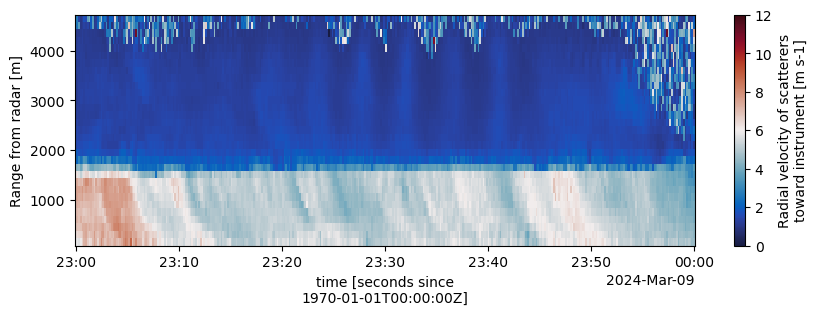
    elevation                    (time) float64 3kB ...

xarray.DataTree

• Groups: (0)
• Dimensions:
  • sample: 64
  • time: 362
  • range: 31
  • index: 11222
• Coordinates: (3)
  • velocity_bins
    (sample)
    float64
    ...

    long_name :

    Doppler velocity bins

    standard_name :

    doppler_velocity_bins

    units :

    m s-1

    [64 values with dtype=float64]

  • range
    (range)
    float64
    150.0 300.0 ... 4.5e+03 4.65e+03

    long_name :

    Range from radar

    standard_name :

    range

    units :

    m

    array([ 150.,  300.,  450.,  600.,  750.,  900., 1050., 1200., 1350., 1500.,
           1650., 1800., 1950., 2100., 2250., 2400., 2550., 2700., 2850., 3000.,
           3150., 3300., 3450., 3600., 3750., 3900., 4050., 4200., 4350., 4500.,
           4650.])

  • time
    (time)
    datetime64[ns]
    2024-03-08T23:00:00 ... 2024-03-...

    standard_name :

    time

    units :

    seconds since 1970-01-01T00:00:00Z

    array(['2024-03-08T23:00:00.000000000', '2024-03-08T23:00:10.000000000',
           '2024-03-08T23:00:20.000000000', ..., '2024-03-08T23:59:37.000000000',
           '2024-03-08T23:59:47.000000000', '2024-03-08T23:59:57.000000000'],
          dtype='datetime64[ns]')

• Inherited coordinates: (0)
• Data variables: (17)
  • transfer_function
    (time, range)
    float64
    ...

    long_name :

    Transfer function

    standard_name :

    transfer_function

    units :

    1

    [11222 values with dtype=float64]

  • spectral_reflectivity
    (index, sample)
    float64
    ...

    long_name :

    Spectral reflectivity

    standard_name :

    equivalent_reflectivity_factor

    units :

    dB

    [718208 values with dtype=float64]

  • drop_size
    (index, sample)
    float64
    ...

    long_name :

    Drop size

    standard_name :

    drop_size

    units :

    mm

    [718208 values with dtype=float64]

  • drop_number_density
    (index, sample)
    float64
    ...

    long_name :

    Raindrop number density

    standard_name :

    raindrop_number_density

    units :

    m-4

    [718208 values with dtype=float64]

  • percentage_valid_spectra
    (time)
    float64
    ...

    long_name :

    Percentage of spectra that are valid

    standard_name :

    percentage_valid_spectra

    units :

    percent

    [362 values with dtype=float64]

  • path_integrated_attenuation
    (time, range)
    float64
    ...

    long_name :

    Path integrated attenuation

    standard_name :

    path_integrated_attenuation

    units :

    dB

    [11222 values with dtype=float64]

  • corrected_reflectivity
    (time, range)
    float64
    ...

    long_name :

    Attenuation-corrected Radar reflectivity factor

    standard_name :

    equivalent_radar_reflectivity_factor

    units :

    dBZ

    [11222 values with dtype=float64]

  • reflectivity
    (time, range)
    float64
    ...

    long_name :

    Radar reflectivity factor

    standard_name :

    equivalent_radar_reflectivity_factor

    units :

    dBZ

    [11222 values with dtype=float64]

  • rainfall_rate
    (time, range)
    float64
    ...

    long_name :

    Rainfall rate

    standard_name :

    rainfall_rate

    units :

    mm hr-1

    [11222 values with dtype=float64]

  • liquid_water_content
    (time, range)
    float64
    ...

    long_name :

    Liquid water content

    standard_name :

    liquid_water_content

    units :

    g m-3

    [11222 values with dtype=float64]

  • velocity
    (time, range)
    float64
    ...

    long_name :

    Radial velocity of scatterers toward instrument

    standard_name :

    radial_velocity_of_scatterers_toward_instrument

    units :

    m s-1

    [11222 values with dtype=float64]

  • altitude
    ()
    float64
    ...

    long_name :

    altitude

    units :

    meters

    standard_name :

    altitude

    [1 values with dtype=float64]

  • longitude
    ()
    float64
    ...

    long_name :

    longitude

    units :

    degrees_east

    standard_name :

    longitude

    [1 values with dtype=float64]

  • latitude
    ()
    float64
    ...

    long_name :

    latitude

    units :

    degrees_north

    positive :

    up

    standard_name :

    latitude

    [1 values with dtype=float64]

  • spectrum_index
    (time, range)
    float64
    ...

    long_name :

    Spectrum index

    standard_name :

    spectrum_index

    units :

    1

    [11222 values with dtype=float64]

  • azimuth
    (time)
    float64
    ...

    standard_name :

    ray_azimuth_angle

    long_name :

    azimuth_angle_from_true_north

    units :

    degrees

    axis :

    radial_azimuth_coordinate

    [362 values with dtype=float64]

  • elevation
    (time)
    float64
    ...

    standard_name :

    ray_elevation_angle

    long_name :

    elevation_angle_from_horizontal_plane

    units :

    degrees

    axis :

    radial_elevation_coordinate

    [362 values with dtype=float64]

• Attributes: (0)

Plot MRR timeseries

One can use the typical xarray plotting functions for plotting the velocity or other MRR2 variables.

plt.figure(figsize=(10, 3))
ds["sweep_0"]["velocity"].T.plot(cmap="balance", vmin=0, vmax=12)

<matplotlib.collections.QuadMesh at 0x7f72ce176570>

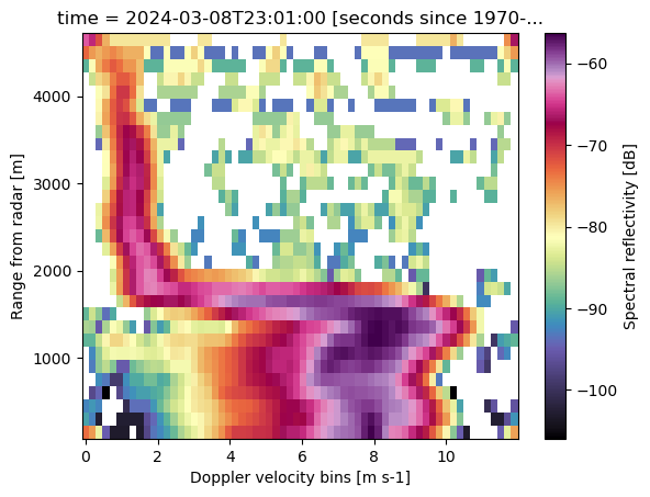
Plot MRR spectra

In order to plot the spectra, you first need to locate the index that corresponds to the given time period. This is done using xarray .sel() functionality to get the indicies.

indicies = ds["sweep_0"]["spectrum_index"].sel(
    time="2024-03-08T23:01:00", method="nearest"
)
indicies
ds["sweep_0"]["spectral_reflectivity"].isel(index=indicies).T.plot(
    cmap="ChaseSpectral", x="velocity_bins"
)

<matplotlib.collections.QuadMesh at 0x7f72ce00ea50>

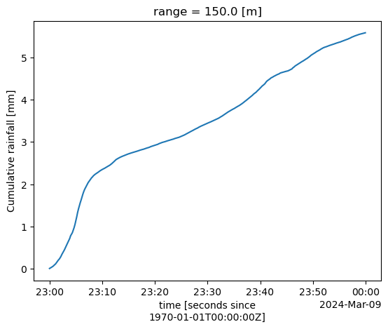
Calculate rainfall accumulation estimated from Doppler velocity spectra

rainfall = ds["sweep_0"]["rainfall_rate"].isel(range=0).cumsum() / 60.0
rainfall.plot()
plt.ylabel("Cumulative rainfall [mm]")

Text(0, 0.5, 'Cumulative rainfall [mm]')