Halo Photonics Doppler Lidar

import matplotlib.pyplot as plt
from open_radar_data import DATASETS

import xradar as xd

Opening a Halo Photonics Doppler lidar .hpl file.

We use the xd.io.open_hpl_datatree in order to load the Halo Photonics Doppler lidar data. After that we will need to enter in the latitude and longitude in order to properly georeference the data. The .hpl file does not contain the latitude, longitude, or altitude of the lidar, so these need to be entered in as keywords as a part of the backend_kwargs argument to xd.io.open_hpl_datatree.

In this example, we are using the coordinates of the Doppler lidar at the Nantucket Wastewater Management Facility, deployed as as part of the DOE Energy Effciency and Renewable Energy Office’s 3rd Wind Forecast Improvement Project.

ds = xd.io.open_hpl_datatree(
    DATASETS.fetch("User1_184_20240601_013257.hpl"),
    sweep=[0, 1, 2, 3, 4, 5, 6, 7, 8],
    backend_kwargs=dict(latitude=41.24276244459537, longitude=-70.1070364814594),
)

Downloading file 'User1_184_20240601_013257.hpl' from 'https://github.com/openradar/open-radar-data/raw/main/data/User1_184_20240601_013257.hpl' to '/home/docs/.cache/open-radar-data'.

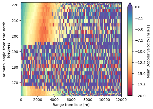
ds["sweep_2"]["mean_doppler_velocity"].plot(vmin=-20, vmax=0, cmap="Spectral")

<matplotlib.collections.QuadMesh at 0x7f6870b9ec30>

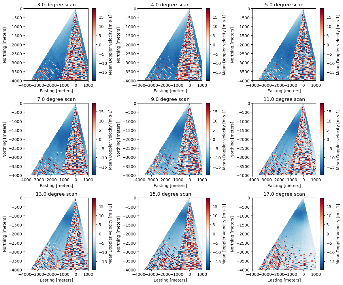
In order to plot each sweep, we need to georeference the underlying sweeps.

fig, ax = plt.subplots(3, 3, figsize=(12, 10))
for sweep in range(9):
    sweep_ds = xd.georeference.get_x_y_z(ds["sweep_%d" % sweep].ds)
    sweep_ds = sweep_ds.set_coords(["x", "y", "z", "time", "range"])
    sweep_ds["mean_doppler_velocity"].plot(
        x="x", y="y", ax=ax[int(sweep / 3), sweep % 3]
    )
    ax[int(sweep / 3), sweep % 3].set_title(
        "{angle:2.1f} degree scan".format(angle=sweep_ds["sweep_fixed_angle"].values)
    )
    ax[int(sweep / 3), sweep % 3].set_ylim([-4000, 0])
    ax[int(sweep / 3), sweep % 3].set_xlim([-4000, 1000])
fig.tight_layout()