Work with AWS#
This example shows how to access radar data from the Colombian national radar network public on Amazon Web Services. We will look at the bucket structure and plot a PPI using the Xradar library. Radar reflectivity is filtered using some polarimetric values and xarray functionality.
Imports#
from datetime import datetime

import boto3
import botocore
import cmweather  # noqa
import fsspec
import matplotlib.pyplot as plt
import xarray as xr
from botocore.client import Config
from pandas import to_datetime

import xradar as xd
IDEAM AWS Bucket#
Instituto de Hidrología, Meteorología y Estudios Ambientales - IDEAM (Colombian National Weather Service) has made public the weather radar data. Data can be found here, and documentation here.
The bucket structure is s3://s3-radaresideam/l2_data/YYYY/MM/DD/Radar_name/RRRAAMMDDTTTTTT.RAWXXXX where:
YYYY is the 4-digit year
MM is the 2-digit month
DD is the 2-digit day
Radar_name radar name. Options are Guaviare, Munchique, Barrancabermja, and Carimagua
RRRAAMMDDTTTTTT.RAWXXXX is the radar filename with the following:
RRR three first letters of the radar name (e.g., GUA for Guaviare radar)
YY is the 2-digit year
MM is the 2-digit month
DD is the 2-digit day
TTTTTT is the time at which the scan was made (GTM)
RAWXXXX Sigmet file format and unique code provided by IRIS software
This is too complicated! No worries. We created a function to help you list files within the bucket.
def create_query(date, radar_site):
    """
    Creates a string for quering the IDEAM radar files stored in AWS bucket
    :param date: date to be queried. e.g datetime(2021, 10, 3, 12). Datetime python object
    :param radar_site: radar site e.g. Guaviare
    :return: string with a IDEAM radar bucket format
    """
    if (date.hour != 0) and (date.minute != 0):
        return f"l2_data/{date:%Y}/{date:%m}/{date:%d}/{radar_site}/{radar_site[:3].upper()}{date:%y%m%d%H%M}"
    elif (date.hour != 0) and (date.minute == 0):
        return f"l2_data/{date:%Y}/{date:%m}/{date:%d}/{radar_site}/{radar_site[:3].upper()}{date:%y%m%d%H}"
    else:
        return f"l2_data/{date:%Y}/{date:%m}/{date:%d}/{radar_site}/{radar_site[:3].upper()}{date:%y%m%d}"
Let’s suppose we want to check the radar files on 2022-10-6 from the Guaviare radar
date_query = datetime(2022, 10, 6)
radar_name = "Guaviare"
query = create_query(date=date_query, radar_site=radar_name)
query
'l2_data/2022/10/06/Guaviare/GUA221006'
Connecting to the AWS bucket#
Once the query is defined, we can procced to list all the available files in the bucket using boto3 and botocore libraries
str_bucket = "s3://s3-radaresideam/"
s3 = boto3.resource(
    "s3",
    config=Config(signature_version=botocore.UNSIGNED, user_agent_extra="Resource"),
)

bucket = s3.Bucket("s3-radaresideam")

radar_files = [f"{str_bucket}{i.key}" for i in bucket.objects.filter(Prefix=f"{query}")]
radar_files[:5]
['s3://s3-radaresideam/l2_data/2022/10/06/Guaviare/GUA221006000012.RAWHDKV',
 's3://s3-radaresideam/l2_data/2022/10/06/Guaviare/GUA221006000116.RAWHDL6',
 's3://s3-radaresideam/l2_data/2022/10/06/Guaviare/GUA221006000248.RAWHDL9',
 's3://s3-radaresideam/l2_data/2022/10/06/Guaviare/GUA221006000327.RAWHDLH',
 's3://s3-radaresideam/l2_data/2022/10/06/Guaviare/GUA221006000432.RAWHDLL']
We can use the Filesystem interfaces for Python fsspec to access the data from the s3 bucket
file = fsspec.open_local(
    f"simplecache::{radar_files[0]}",
    s3={"anon": True},
    filecache={"cache_storage": "."},
)
/home/docs/checkouts/readthedocs.org/user_builds/xradar/conda/latest/lib/python3.13/site-packages/fsspec/registry.py:305: UserWarning: Your installed version of s3fs is very old and known to cause
severe performance issues, see also https://github.com/dask/dask/issues/10276

To fix, you should specify a lower version bound on s3fs, or
update the current installation.

  warnings.warn(s3_msg)
ds = xr.open_dataset(file, engine="iris", group="sweep_0")
display(ds)
<xarray.Dataset> Size: 33MB
Dimensions:            (azimuth: 720, range: 994)
Coordinates:
  * azimuth            (azimuth) float32 3kB 0.02747 0.5191 ... 359.0 359.5
    elevation          (azimuth) float32 3kB ...
    time               (azimuth) datetime64[ns] 6kB ...
  * range              (range) float32 4kB 1e+03 1.3e+03 ... 2.986e+05 2.989e+05
    longitude          float64 8B ...
    latitude           float64 8B ...
    altitude           float64 8B ...
Data variables: (12/17)
    DBTH               (azimuth, range) float32 3MB ...
    DBZH               (azimuth, range) float32 3MB ...
    VRADH              (azimuth, range) float32 3MB ...
    WRADH              (azimuth, range) float32 3MB ...
    ZDR                (azimuth, range) float32 3MB ...
    KDP                (azimuth, range) float32 3MB ...
    ...                 ...
    DB_DBZE8           (azimuth, range) float32 3MB ...
    sweep_mode         <U20 80B ...
    sweep_number       int64 8B ...
    prt_mode           <U7 28B ...
    follow_mode        <U7 28B ...
    sweep_fixed_angle  float64 8B ...
Attributes:
    source:           Sigmet
    scan_name:        SURVP
    instrument_name:  guaviare
comment: Primera tarea del modo procipitacion / 0.5Reflectivity and Correlation coefficient plot#
fig, (ax, ax1) = plt.subplots(1, 2, figsize=(10, 4), dpi=120)
ds.DBZH.plot(cmap="ChaseSpectral", vmin=-10, vmax=50, ax=ax)
ds.RHOHV.plot(cmap="ChaseSpectral", vmin=0, vmax=1, ax=ax1)
fig.tight_layout()
/home/docs/checkouts/readthedocs.org/user_builds/xradar/conda/latest/lib/python3.13/site-packages/xradar/io/backends/iris.py:254: RuntimeWarning: invalid value encountered in sqrt
  return np.sqrt(decode_array(data, **kwargs))
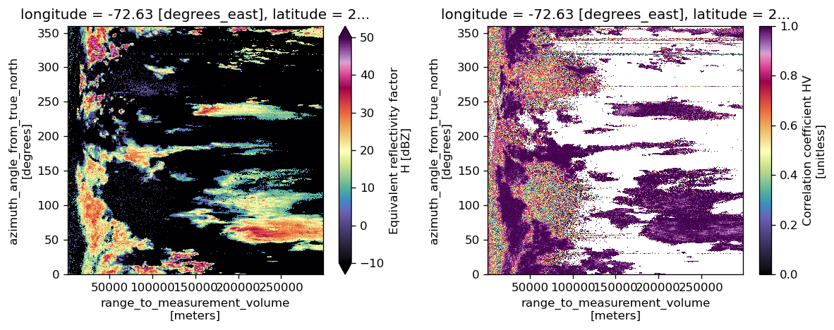
The dataset object has range and azimuth as coordinates. To create a polar plot, we need to add the georeference information using xd.georeference.get_x_y_z() module from xradar
ds = xd.georeference.get_x_y_z(ds)
display(ds)
<xarray.Dataset> Size: 50MB
Dimensions:            (azimuth: 720, range: 994)
Coordinates:
  * azimuth            (azimuth) float32 3kB 0.02747 0.5191 ... 359.0 359.5
    elevation          (azimuth) float64 6kB 0.4834 0.4834 ... 0.4834 0.4834
    time               (azimuth) datetime64[ns] 6kB ...
  * range              (range) float32 4kB 1e+03 1.3e+03 ... 2.986e+05 2.989e+05
    x                  (azimuth, range) float64 6MB 0.4793 0.6231 ... -2.491e+03
    y                  (azimuth, range) float64 6MB 999.9 1.3e+03 ... 2.987e+05
    z                  (azimuth, range) float64 6MB 248.5 251.1 ... 8.011e+03
    longitude          float64 8B -72.63
    latitude           float64 8B 2.534
    altitude           float64 8B 240.0
    crs_wkt            int64 8B 0
Data variables: (12/17)
    DBTH               (azimuth, range) float32 3MB ...
    DBZH               (azimuth, range) float32 3MB ...
    VRADH              (azimuth, range) float32 3MB ...
    WRADH              (azimuth, range) float32 3MB ...
    ZDR                (azimuth, range) float32 3MB ...
    KDP                (azimuth, range) float32 3MB ...
    ...                 ...
    DB_DBZE8           (azimuth, range) float32 3MB ...
    sweep_mode         <U20 80B ...
    sweep_number       int64 8B ...
    prt_mode           <U7 28B ...
    follow_mode        <U7 28B ...
    sweep_fixed_angle  float64 8B ...
Attributes:
    source:           Sigmet
    scan_name:        SURVP
    instrument_name:  guaviare
comment: Primera tarea del modo procipitacion / 0.5Now x, y, and z have been added to the dataset coordinates. Let’s create the new plot using the georeference information.
fig, (ax, ax1) = plt.subplots(1, 2, figsize=(10, 4))
ds.DBZH.plot(x="x", y="y", cmap="ChaseSpectral", vmin=-10, vmax=50, ax=ax)
ds.RHOHV.plot(x="x", y="y", cmap="ChaseSpectral", vmin=0, vmax=1, ax=ax1)
ax.set_title("")
ax1.set_title("")
fig.tight_layout()
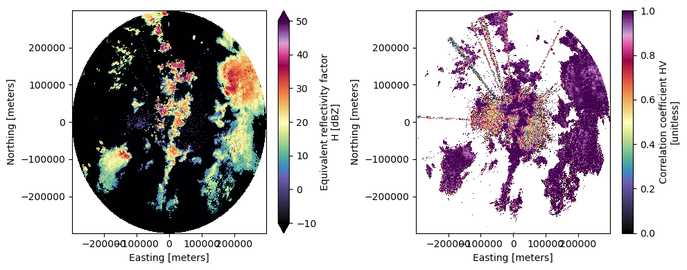
Filtering data#
The blue background color indicates that the radar reflectivity is less than -10 dBZ. we can filter radar data using xarray.where module
fig, (ax, ax1) = plt.subplots(1, 2, figsize=(10, 4))
ds.DBZH.where(ds.DBZH >= -10).plot(
    x="x", y="y", cmap="ChaseSpectral", vmin=-10, vmax=50, ax=ax
)
ds.RHOHV.where(ds.DBZH >= -10).plot(
    x="x", y="y", cmap="ChaseSpectral", vmin=0, vmax=1, ax=ax1
)
ax.set_title("")
ax1.set_title("")
fig.tight_layout()
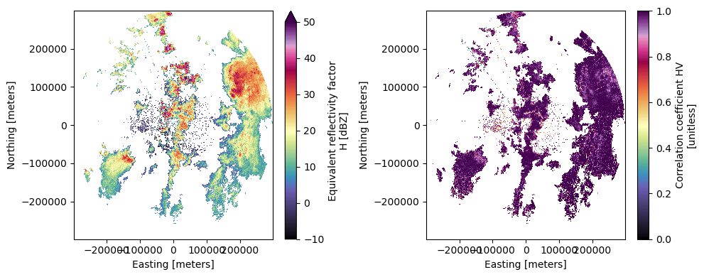
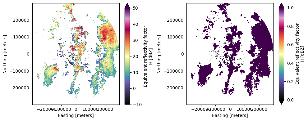
Polarimetric variables can also be used as indicators to remove different noises from different sources. For example, the \(\rho_{HV}\) measures the consistency of the shapes and sizes of targets within the radar beam. Thus, the greater the \(\rho_{HV}\), the more consistent the measurement. For this example we can use \(\rho_{HV} > 0.80\) as an acceptable threshold
fig, (ax, ax1) = plt.subplots(1, 2, figsize=(10, 4))
ds.DBZH.where(ds.DBZH >= -10).where(ds.RHOHV >= 0.80).plot(
    x="x", y="y", cmap="ChaseSpectral", vmin=-10, vmax=50, ax=ax
)

ds.DBZH.where(ds.DBZH >= -10).where(ds.RHOHV >= 0.85).plot(
    x="x", y="y", cmap="ChaseSpectral", vmin=0, vmax=1, ax=ax1
)
ax.set_title("")
ax1.set_title("")
fig.tight_layout()
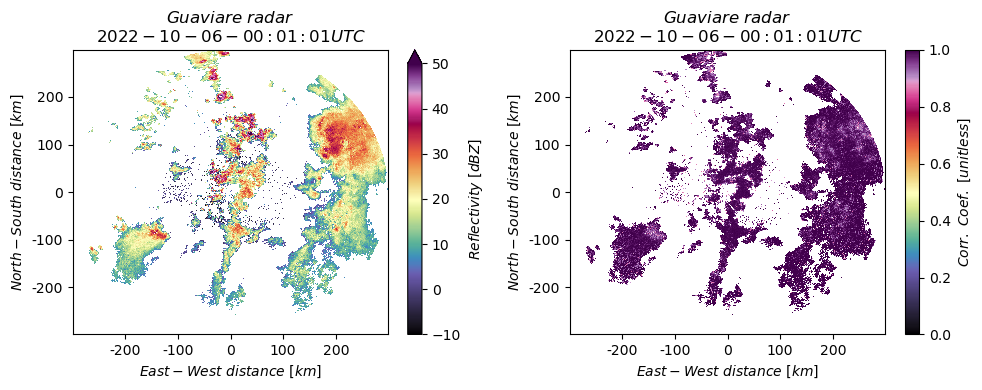
Axis labels and titles#
We can change some axis labels as well as the colorbar label
fig, (ax, ax1) = plt.subplots(1, 2, figsize=(10, 4))
ds.DBZH.where(ds.DBZH >= -10).where(ds.RHOHV >= 0.85).plot(
    x="x",
    y="y",
    cmap="ChaseSpectral",
    vmin=-10,
    vmax=50,
    ax=ax,
    cbar_kwargs={"label": r"$Reflectivity \ [dBZ]$"},
)

ds.RHOHV.where(ds.DBZH >= -10).where(ds.RHOHV >= 0.85).plot(
    x="x",
    y="y",
    cmap="ChaseSpectral",
    vmin=0,
    vmax=1,
    ax=ax1,
    cbar_kwargs={"label": r"$Corr. \ Coef. \  [unitless]$"},
)

# lambda fucntion for unit trasformation m->km
m2km = lambda x, _: f"{x/1000:g}"
# set new ticks
ax.xaxis.set_major_formatter(m2km)
ax.yaxis.set_major_formatter(m2km)
ax1.xaxis.set_major_formatter(m2km)
ax1.yaxis.set_major_formatter(m2km)
# removing the title in both plots
ax.set_title("")
ax1.set_title("")

# renaming the axis
ax.set_ylabel(r"$North - South \ distance \ [km]$")
ax.set_xlabel(r"$East - West \ distance \ [km]$")
ax1.set_ylabel(r"$North - South \ distance \ [km]$")
ax1.set_xlabel(r"$East - West \ distance \ [km]$")

# setting up the title
ax.set_title(
    r"$Guaviare \ radar$"
    + "\n"
    + f"${to_datetime(ds.time.values[0]): %Y-%m-%d - %X}$"
    + "$ UTC$"
)
ax1.set_title(
    r"$Guaviare \ radar$"
    + "\n"
    + f"${to_datetime(ds.time.values[0]): %Y-%m-%d - %X}$"
    + "$ UTC$"
)
fig.tight_layout()