Plan Position Indicator#
A Plan Position Indicator (PPI) plot is a common plot requested by radar scientists. Let’s show how to create this plot using xradar
Imports#
import cmweather  # noqa
from open_radar_data import DATASETS

import xradar as xd
import cartopy
import matplotlib.pyplot as plt
Read in some data#
Fetching CfRadial1 radar data file from open-radar-data repository.
filename = DATASETS.fetch("cfrad.20080604_002217_000_SPOL_v36_SUR.nc")
Read the data using the cfradial1 engine
radar = xd.io.open_cfradial1_datatree(filename, first_dim="auto")
display(radar)
<xarray.DataTree>
Group: /
│   Dimensions:              (sweep: 9)
│   Coordinates:
│       latitude             float64 8B ...
│       longitude            float64 8B ...
│       altitude             float64 8B ...
│   Dimensions without coordinates: sweep
│   Data variables:
│       volume_number        int32 4B ...
│       platform_type        |S32 32B ...
│       primary_axis         |S32 32B ...
│       status_str           |S1 1B ...
│       instrument_type      |S32 32B ...
│       time_coverage_start  |S32 32B ...
│       time_coverage_end    |S32 32B ...
│       sweep_group_name     (sweep) <U7 252B 'sweep_0' 'sweep_1' ... 'sweep_8'
│       sweep_fixed_angle    (sweep) float32 36B ...
│   Attributes: (12/13)
│       Conventions:         CF/Radial instrument_parameters radar_parameters rad...
│       version:             1.2
│       title:               TIMREX
│       institution:
│       references:
│       source:
│       ...                  ...
│       comment:
│       instrument_name:     SPOLRVP8
│       site_name:
│       scan_name:
│       scan_id:             0
│       platform_is_mobile:  false
├── Group: /sweep_0
│       Dimensions:                    (azimuth: 483, range: 996)
│       Coordinates:
│         * azimuth                    (azimuth) float32 2kB 0.0 0.75 ... 358.5 359.2
│           elevation                  (azimuth) float32 2kB ...
│           time                       (azimuth) datetime64[ns] 4kB 2008-06-04T00:15:...
│         * range                      (range) float32 4kB 150.0 300.0 ... 1.494e+05
│       Data variables: (12/18)
│           sweep_number               int32 4B ...
│           sweep_mode                 <U20 80B 'azimuth_surveillance'
│           prt_mode                   |S32 32B ...
│           follow_mode                |S32 32B ...
│           sweep_fixed_angle          float32 4B ...
│           pulse_width                (azimuth) float32 2kB ...
│           ...                         ...
│           r_calib_index              (azimuth) int8 483B ...
│           measured_transmit_power_h  (azimuth) float32 2kB ...
│           measured_transmit_power_v  (azimuth) float32 2kB ...
│           scan_rate                  (azimuth) float32 2kB ...
│           DBZ                        (azimuth, range) float32 2MB ...
│           VR                         (azimuth, range) float32 2MB ...
├── Group: /sweep_1
│       Dimensions:                    (azimuth: 483, range: 996)
│       Coordinates:
│         * azimuth                    (azimuth) float32 2kB 0.0 0.75 ... 358.5 359.2
│           elevation                  (azimuth) float32 2kB ...
│           time                       (azimuth) datetime64[ns] 4kB 2008-06-04T00:16:...
│         * range                      (range) float32 4kB 150.0 300.0 ... 1.494e+05
│       Data variables: (12/18)
│           sweep_number               int32 4B ...
│           sweep_mode                 <U20 80B 'azimuth_surveillance'
│           prt_mode                   |S32 32B ...
│           follow_mode                |S32 32B ...
│           sweep_fixed_angle          float32 4B ...
│           pulse_width                (azimuth) float32 2kB ...
│           ...                         ...
│           r_calib_index              (azimuth) int8 483B ...
│           measured_transmit_power_h  (azimuth) float32 2kB ...
│           measured_transmit_power_v  (azimuth) float32 2kB ...
│           scan_rate                  (azimuth) float32 2kB ...
│           DBZ                        (azimuth, range) float32 2MB ...
│           VR                         (azimuth, range) float32 2MB ...
├── Group: /sweep_2
│       Dimensions:                    (azimuth: 482, range: 996)
│       Coordinates:
│         * azimuth                    (azimuth) float32 2kB 0.0 0.75 ... 358.5 359.2
│           elevation                  (azimuth) float32 2kB ...
│           time                       (azimuth) datetime64[ns] 4kB 2008-06-04T00:17:...
│         * range                      (range) float32 4kB 150.0 300.0 ... 1.494e+05
│       Data variables: (12/18)
│           sweep_number               int32 4B ...
│           sweep_mode                 <U20 80B 'azimuth_surveillance'
│           prt_mode                   |S32 32B ...
│           follow_mode                |S32 32B ...
│           sweep_fixed_angle          float32 4B ...
│           pulse_width                (azimuth) float32 2kB ...
│           ...                         ...
│           r_calib_index              (azimuth) int8 482B ...
│           measured_transmit_power_h  (azimuth) float32 2kB ...
│           measured_transmit_power_v  (azimuth) float32 2kB ...
│           scan_rate                  (azimuth) float32 2kB ...
│           DBZ                        (azimuth, range) float32 2MB ...
│           VR                         (azimuth, range) float32 2MB ...
├── Group: /sweep_3
│       Dimensions:                    (azimuth: 483, range: 996)
│       Coordinates:
│         * azimuth                    (azimuth) float32 2kB 0.0 0.75 ... 358.5 359.2
│           elevation                  (azimuth) float32 2kB ...
│           time                       (azimuth) datetime64[ns] 4kB 2008-06-04T00:17:...
│         * range                      (range) float32 4kB 150.0 300.0 ... 1.494e+05
│       Data variables: (12/18)
│           sweep_number               int32 4B ...
│           sweep_mode                 <U20 80B 'azimuth_surveillance'
│           prt_mode                   |S32 32B ...
│           follow_mode                |S32 32B ...
│           sweep_fixed_angle          float32 4B ...
│           pulse_width                (azimuth) float32 2kB ...
│           ...                         ...
│           r_calib_index              (azimuth) int8 483B ...
│           measured_transmit_power_h  (azimuth) float32 2kB ...
│           measured_transmit_power_v  (azimuth) float32 2kB ...
│           scan_rate                  (azimuth) float32 2kB ...
│           DBZ                        (azimuth, range) float32 2MB ...
│           VR                         (azimuth, range) float32 2MB ...
├── Group: /sweep_4
│       Dimensions:                    (azimuth: 481, range: 996)
│       Coordinates:
│         * azimuth                    (azimuth) float32 2kB 0.0 0.75 ... 358.5 359.2
│           elevation                  (azimuth) float32 2kB ...
│           time                       (azimuth) datetime64[ns] 4kB 2008-06-04T00:18:...
│         * range                      (range) float32 4kB 150.0 300.0 ... 1.494e+05
│       Data variables: (12/18)
│           sweep_number               int32 4B ...
│           sweep_mode                 <U20 80B 'azimuth_surveillance'
│           prt_mode                   |S32 32B ...
│           follow_mode                |S32 32B ...
│           sweep_fixed_angle          float32 4B ...
│           pulse_width                (azimuth) float32 2kB ...
│           ...                         ...
│           r_calib_index              (azimuth) int8 481B ...
│           measured_transmit_power_h  (azimuth) float32 2kB ...
│           measured_transmit_power_v  (azimuth) float32 2kB ...
│           scan_rate                  (azimuth) float32 2kB ...
│           DBZ                        (azimuth, range) float32 2MB ...
│           VR                         (azimuth, range) float32 2MB ...
├── Group: /sweep_5
│       Dimensions:                    (azimuth: 482, range: 996)
│       Coordinates:
│         * azimuth                    (azimuth) float32 2kB 0.0 0.75 ... 358.5 359.2
│           elevation                  (azimuth) float32 2kB ...
│           time                       (azimuth) datetime64[ns] 4kB 2008-06-04T00:19:...
│         * range                      (range) float32 4kB 150.0 300.0 ... 1.494e+05
│       Data variables: (12/18)
│           sweep_number               int32 4B ...
│           sweep_mode                 <U20 80B 'azimuth_surveillance'
│           prt_mode                   |S32 32B ...
│           follow_mode                |S32 32B ...
│           sweep_fixed_angle          float32 4B ...
│           pulse_width                (azimuth) float32 2kB ...
│           ...                         ...
│           r_calib_index              (azimuth) int8 482B ...
│           measured_transmit_power_h  (azimuth) float32 2kB ...
│           measured_transmit_power_v  (azimuth) float32 2kB ...
│           scan_rate                  (azimuth) float32 2kB ...
│           DBZ                        (azimuth, range) float32 2MB ...
│           VR                         (azimuth, range) float32 2MB ...
├── Group: /sweep_6
│       Dimensions:                    (azimuth: 482, range: 996)
│       Coordinates:
│         * azimuth                    (azimuth) float32 2kB 0.0 0.75 ... 358.5 359.2
│           elevation                  (azimuth) float32 2kB ...
│           time                       (azimuth) datetime64[ns] 4kB 2008-06-04T00:20:...
│         * range                      (range) float32 4kB 150.0 300.0 ... 1.494e+05
│       Data variables: (12/18)
│           sweep_number               int32 4B ...
│           sweep_mode                 <U20 80B 'azimuth_surveillance'
│           prt_mode                   |S32 32B ...
│           follow_mode                |S32 32B ...
│           sweep_fixed_angle          float32 4B ...
│           pulse_width                (azimuth) float32 2kB ...
│           ...                         ...
│           r_calib_index              (azimuth) int8 482B ...
│           measured_transmit_power_h  (azimuth) float32 2kB ...
│           measured_transmit_power_v  (azimuth) float32 2kB ...
│           scan_rate                  (azimuth) float32 2kB ...
│           DBZ                        (azimuth, range) float32 2MB ...
│           VR                         (azimuth, range) float32 2MB ...
├── Group: /sweep_7
│       Dimensions:                    (azimuth: 484, range: 996)
│       Coordinates:
│         * azimuth                    (azimuth) float32 2kB 0.0 0.75 ... 358.5 359.2
│           elevation                  (azimuth) float32 2kB ...
│           time                       (azimuth) datetime64[ns] 4kB 2008-06-04T00:21:...
│         * range                      (range) float32 4kB 150.0 300.0 ... 1.494e+05
│       Data variables: (12/18)
│           sweep_number               int32 4B ...
│           sweep_mode                 <U20 80B 'azimuth_surveillance'
│           prt_mode                   |S32 32B ...
│           follow_mode                |S32 32B ...
│           sweep_fixed_angle          float32 4B ...
│           pulse_width                (azimuth) float32 2kB ...
│           ...                         ...
│           r_calib_index              (azimuth) int8 484B ...
│           measured_transmit_power_h  (azimuth) float32 2kB ...
│           measured_transmit_power_v  (azimuth) float32 2kB ...
│           scan_rate                  (azimuth) float32 2kB ...
│           DBZ                        (azimuth, range) float32 2MB ...
│           VR                         (azimuth, range) float32 2MB ...
└── Group: /sweep_8
        Dimensions:                    (azimuth: 483, range: 996)
        Coordinates:
          * azimuth                    (azimuth) float32 2kB 0.0 0.75 ... 358.5 359.2
            elevation                  (azimuth) float32 2kB ...
            time                       (azimuth) datetime64[ns] 4kB 2008-06-04T00:21:...
          * range                      (range) float32 4kB 150.0 300.0 ... 1.494e+05
        Data variables: (12/18)
            sweep_number               int32 4B ...
            sweep_mode                 <U20 80B 'azimuth_surveillance'
            prt_mode                   |S32 32B ...
            follow_mode                |S32 32B ...
            sweep_fixed_angle          float32 4B ...
            pulse_width                (azimuth) float32 2kB ...
            ...                         ...
            r_calib_index              (azimuth) int8 483B ...
            measured_transmit_power_h  (azimuth) float32 2kB ...
            measured_transmit_power_v  (azimuth) float32 2kB ...
            scan_rate                  (azimuth) float32 2kB ...
            DBZ                        (azimuth, range) float32 2MB ...
VR (azimuth, range) float32 2MB ...Add georeferencing#
We can use the georeference function, or the accessor to add our georeference information!
Georeference Accessor#
If you prefer the accessor (.xradar.georefence()), this is how you would add georeference information to your radar object.
radar = radar.xradar.georeference()
display(radar)
<xarray.DataTree>
Group: /
│ Dimensions: (sweep: 9)
│ Coordinates:
│ latitude float64 8B ...
│ longitude float64 8B ...
│ altitude float64 8B ...
│ Dimensions without coordinates: sweep
│ Data variables:
│ volume_number int32 4B ...
│ platform_type |S32 32B ...
│ primary_axis |S32 32B ...
│ status_str |S1 1B ...
│ instrument_type |S32 32B ...
│ time_coverage_start |S32 32B ...
│ time_coverage_end |S32 32B ...
│ sweep_group_name (sweep) <U7 252B 'sweep_0' 'sweep_1' ... 'sweep_8'
│ sweep_fixed_angle (sweep) float32 36B ...
│ Attributes: (12/13)
│ Conventions: CF/Radial instrument_parameters radar_parameters rad...
│ version: 1.2
│ title: TIMREX
│ institution:
│ references:
│ source:
│ ... ...
│ comment:
│ instrument_name: SPOLRVP8
│ site_name:
│ scan_name:
│ scan_id: 0
│ platform_is_mobile: false
├── Group: /sweep_0
│ Dimensions: (azimuth: 483, range: 996)
│ Coordinates:
│ * azimuth (azimuth) float32 2kB 0.0 0.75 ... 358.5 359.2
│ elevation (azimuth) float32 2kB 0.5164 0.5219 ... 0.5219
│ time (azimuth) datetime64[ns] 4kB 2008-06-04T00:15:...
│ * range (range) float32 4kB 150.0 300.0 ... 1.494e+05
│ x (azimuth, range) float64 4MB 0.0 ... -1.955e+03
│ y (azimuth, range) float64 4MB 150.0 ... 1.493e+05
│ z (azimuth, range) float64 4MB 46.35 ... 2.718e+03
│ latitude float64 8B 22.53
│ longitude float64 8B 120.4
│ altitude float64 8B 45.0
│ crs_wkt int64 8B 0
│ Data variables: (12/18)
│ sweep_number int32 4B ...
│ sweep_mode <U20 80B 'azimuth_surveillance'
│ prt_mode |S32 32B ...
│ follow_mode |S32 32B ...
│ sweep_fixed_angle float32 4B ...
│ pulse_width (azimuth) float32 2kB ...
│ ... ...
│ r_calib_index (azimuth) int8 483B ...
│ measured_transmit_power_h (azimuth) float32 2kB ...
│ measured_transmit_power_v (azimuth) float32 2kB ...
│ scan_rate (azimuth) float32 2kB ...
│ DBZ (azimuth, range) float32 2MB ...
│ VR (azimuth, range) float32 2MB ...
├── Group: /sweep_1
│ Dimensions: (azimuth: 483, range: 996)
│ Coordinates:
│ * azimuth (azimuth) float32 2kB 0.0 0.75 ... 358.5 359.2
│ elevation (azimuth) float32 2kB 1.104 1.104 ... 1.104 1.104
│ time (azimuth) datetime64[ns] 4kB 2008-06-04T00:16:...
│ * range (range) float32 4kB 150.0 300.0 ... 1.494e+05
│ x (azimuth, range) float64 4MB 0.0 ... -1.954e+03
│ y (azimuth, range) float64 4MB 150.0 ... 1.493e+05
│ z (azimuth, range) float64 4MB 47.89 ... 4.236e+03
│ latitude float64 8B 22.53
│ longitude float64 8B 120.4
│ altitude float64 8B 45.0
│ crs_wkt int64 8B 0
│ Data variables: (12/18)
│ sweep_number int32 4B ...
│ sweep_mode <U20 80B 'azimuth_surveillance'
│ prt_mode |S32 32B ...
│ follow_mode |S32 32B ...
│ sweep_fixed_angle float32 4B ...
│ pulse_width (azimuth) float32 2kB ...
│ ... ...
│ r_calib_index (azimuth) int8 483B ...
│ measured_transmit_power_h (azimuth) float32 2kB ...
│ measured_transmit_power_v (azimuth) float32 2kB ...
│ scan_rate (azimuth) float32 2kB ...
│ DBZ (azimuth, range) float32 2MB ...
│ VR (azimuth, range) float32 2MB ...
├── Group: /sweep_2
│ Dimensions: (azimuth: 482, range: 996)
│ Coordinates:
│ * azimuth (azimuth) float32 2kB 0.0 0.75 ... 358.5 359.2
│ elevation (azimuth) float32 2kB 1.796 1.796 ... 1.796 1.796
│ time (azimuth) datetime64[ns] 4kB 2008-06-04T00:17:...
│ * range (range) float32 4kB 150.0 300.0 ... 1.494e+05
│ x (azimuth, range) float64 4MB 0.0 ... -1.953e+03
│ y (azimuth, range) float64 4MB 149.9 ... 1.492e+05
│ z (azimuth, range) float64 4MB 49.7 ... 6.039e+03
│ latitude float64 8B 22.53
│ longitude float64 8B 120.4
│ altitude float64 8B 45.0
│ crs_wkt int64 8B 0
│ Data variables: (12/18)
│ sweep_number int32 4B ...
│ sweep_mode <U20 80B 'azimuth_surveillance'
│ prt_mode |S32 32B ...
│ follow_mode |S32 32B ...
│ sweep_fixed_angle float32 4B ...
│ pulse_width (azimuth) float32 2kB ...
│ ... ...
│ r_calib_index (azimuth) int8 482B ...
│ measured_transmit_power_h (azimuth) float32 2kB ...
│ measured_transmit_power_v (azimuth) float32 2kB ...
│ scan_rate (azimuth) float32 2kB ...
│ DBZ (azimuth, range) float32 2MB ...
│ VR (azimuth, range) float32 2MB ...
├── Group: /sweep_3
│ Dimensions: (azimuth: 483, range: 996)
│ Coordinates:
│ * azimuth (azimuth) float32 2kB 0.0 0.75 ... 358.5 359.2
│ elevation (azimuth) float32 2kB 2.598 2.598 ... 2.598 2.598
│ time (azimuth) datetime64[ns] 4kB 2008-06-04T00:17:...
│ * range (range) float32 4kB 150.0 300.0 ... 1.494e+05
│ x (azimuth, range) float64 4MB 0.0 ... -1.952e+03
│ y (azimuth, range) float64 4MB 149.8 ... 1.491e+05
│ z (azimuth, range) float64 4MB 51.8 ... 8.127e+03
│ latitude float64 8B 22.53
│ longitude float64 8B 120.4
│ altitude float64 8B 45.0
│ crs_wkt int64 8B 0
│ Data variables: (12/18)
│ sweep_number int32 4B ...
│ sweep_mode <U20 80B 'azimuth_surveillance'
│ prt_mode |S32 32B ...
│ follow_mode |S32 32B ...
│ sweep_fixed_angle float32 4B ...
│ pulse_width (azimuth) float32 2kB ...
│ ... ...
│ r_calib_index (azimuth) int8 483B ...
│ measured_transmit_power_h (azimuth) float32 2kB ...
│ measured_transmit_power_v (azimuth) float32 2kB ...
│ scan_rate (azimuth) float32 2kB ...
│ DBZ (azimuth, range) float32 2MB ...
│ VR (azimuth, range) float32 2MB ...
├── Group: /sweep_4
│ Dimensions: (azimuth: 481, range: 996)
│ Coordinates:
│ * azimuth (azimuth) float32 2kB 0.0 0.75 ... 358.5 359.2
│ elevation (azimuth) float32 2kB 3.598 3.598 ... 3.598 3.598
│ time (azimuth) datetime64[ns] 4kB 2008-06-04T00:18:...
│ * range (range) float32 4kB 150.0 300.0 ... 1.494e+05
│ x (azimuth, range) float64 4MB 0.0 ... -1.949e+03
│ y (azimuth, range) float64 4MB 149.7 ... 1.489e+05
│ z (azimuth, range) float64 4MB 54.41 ... 1.073e+04
│ latitude float64 8B 22.53
│ longitude float64 8B 120.4
│ altitude float64 8B 45.0
│ crs_wkt int64 8B 0
│ Data variables: (12/18)
│ sweep_number int32 4B ...
│ sweep_mode <U20 80B 'azimuth_surveillance'
│ prt_mode |S32 32B ...
│ follow_mode |S32 32B ...
│ sweep_fixed_angle float32 4B ...
│ pulse_width (azimuth) float32 2kB ...
│ ... ...
│ r_calib_index (azimuth) int8 481B ...
│ measured_transmit_power_h (azimuth) float32 2kB ...
│ measured_transmit_power_v (azimuth) float32 2kB ...
│ scan_rate (azimuth) float32 2kB ...
│ DBZ (azimuth, range) float32 2MB ...
│ VR (azimuth, range) float32 2MB ...
├── Group: /sweep_5
│ Dimensions: (azimuth: 482, range: 996)
│ Coordinates:
│ * azimuth (azimuth) float32 2kB 0.0 0.75 ... 358.5 359.2
│ elevation (azimuth) float32 2kB 4.708 4.708 ... 4.708 4.708
│ time (azimuth) datetime64[ns] 4kB 2008-06-04T00:19:...
│ * range (range) float32 4kB 150.0 300.0 ... 1.494e+05
│ x (azimuth, range) float64 4MB 0.0 ... -1.946e+03
│ y (azimuth, range) float64 4MB 149.5 ... 1.487e+05
│ z (azimuth, range) float64 4MB 57.31 ... 1.361e+04
│ latitude float64 8B 22.53
│ longitude float64 8B 120.4
│ altitude float64 8B 45.0
│ crs_wkt int64 8B 0
│ Data variables: (12/18)
│ sweep_number int32 4B ...
│ sweep_mode <U20 80B 'azimuth_surveillance'
│ prt_mode |S32 32B ...
│ follow_mode |S32 32B ...
│ sweep_fixed_angle float32 4B ...
│ pulse_width (azimuth) float32 2kB ...
│ ... ...
│ r_calib_index (azimuth) int8 482B ...
│ measured_transmit_power_h (azimuth) float32 2kB ...
│ measured_transmit_power_v (azimuth) float32 2kB ...
│ scan_rate (azimuth) float32 2kB ...
│ DBZ (azimuth, range) float32 2MB ...
│ VR (azimuth, range) float32 2MB ...
├── Group: /sweep_6
│ Dimensions: (azimuth: 482, range: 996)
│ Coordinates:
│ * azimuth (azimuth) float32 2kB 0.0 0.75 ... 358.5 359.2
│ elevation (azimuth) float32 2kB 6.471 6.471 ... 6.471 6.471
│ time (azimuth) datetime64[ns] 4kB 2008-06-04T00:20:...
│ * range (range) float32 4kB 150.0 300.0 ... 1.494e+05
│ x (azimuth, range) float64 4MB 0.0 ... -1.939e+03
│ y (azimuth, range) float64 4MB 149.0 ... 1.481e+05
│ z (azimuth, range) float64 4MB 61.91 ... 1.818e+04
│ latitude float64 8B 22.53
│ longitude float64 8B 120.4
│ altitude float64 8B 45.0
│ crs_wkt int64 8B 0
│ Data variables: (12/18)
│ sweep_number int32 4B ...
│ sweep_mode <U20 80B 'azimuth_surveillance'
│ prt_mode |S32 32B ...
│ follow_mode |S32 32B ...
│ sweep_fixed_angle float32 4B ...
│ pulse_width (azimuth) float32 2kB ...
│ ... ...
│ r_calib_index (azimuth) int8 482B ...
│ measured_transmit_power_h (azimuth) float32 2kB ...
│ measured_transmit_power_v (azimuth) float32 2kB ...
│ scan_rate (azimuth) float32 2kB ...
│ DBZ (azimuth, range) float32 2MB ...
│ VR (azimuth, range) float32 2MB ...
├── Group: /sweep_7
│ Dimensions: (azimuth: 484, range: 996)
│ Coordinates:
│ * azimuth (azimuth) float32 2kB 0.0 0.75 ... 358.5 359.2
│ elevation (azimuth) float32 2kB 9.102 9.102 ... 9.102 9.102
│ time (azimuth) datetime64[ns] 4kB 2008-06-04T00:21:...
│ * range (range) float32 4kB 150.0 300.0 ... 1.494e+05
│ x (azimuth, range) float64 4MB 0.0 ... -1.925e+03
│ y (azimuth, range) float64 4MB 148.1 ... 1.471e+05
│ z (azimuth, range) float64 4MB 68.73 ... 2.496e+04
│ latitude float64 8B 22.53
│ longitude float64 8B 120.4
│ altitude float64 8B 45.0
│ crs_wkt int64 8B 0
│ Data variables: (12/18)
│ sweep_number int32 4B ...
│ sweep_mode <U20 80B 'azimuth_surveillance'
│ prt_mode |S32 32B ...
│ follow_mode |S32 32B ...
│ sweep_fixed_angle float32 4B ...
│ pulse_width (azimuth) float32 2kB ...
│ ... ...
│ r_calib_index (azimuth) int8 484B ...
│ measured_transmit_power_h (azimuth) float32 2kB ...
│ measured_transmit_power_v (azimuth) float32 2kB ...
│ scan_rate (azimuth) float32 2kB ...
│ DBZ (azimuth, range) float32 2MB ...
│ VR (azimuth, range) float32 2MB ...
└── Group: /sweep_8
Dimensions: (azimuth: 483, range: 996)
Coordinates:
* azimuth (azimuth) float32 2kB 0.0 0.75 ... 358.5 359.2
elevation (azimuth) float32 2kB 12.8 12.8 ... 12.79 12.8
time (azimuth) datetime64[ns] 4kB 2008-06-04T00:21:...
* range (range) float32 4kB 150.0 300.0 ... 1.494e+05
x (azimuth, range) float64 4MB 0.0 ... -1.899e+03
y (azimuth, range) float64 4MB 146.3 ... 1.451e+05
z (azimuth, range) float64 4MB 78.23 ... 3.439e+04
latitude float64 8B 22.53
longitude float64 8B 120.4
altitude float64 8B 45.0
crs_wkt int64 8B 0
Data variables: (12/18)
sweep_number int32 4B ...
sweep_mode <U20 80B 'azimuth_surveillance'
prt_mode |S32 32B ...
follow_mode |S32 32B ...
sweep_fixed_angle float32 4B ...
pulse_width (azimuth) float32 2kB ...
... ...
r_calib_index (azimuth) int8 483B ...
measured_transmit_power_h (azimuth) float32 2kB ...
measured_transmit_power_v (azimuth) float32 2kB ...
scan_rate (azimuth) float32 2kB ...
DBZ (azimuth, range) float32 2MB ...
VR (azimuth, range) float32 2MB ...Please observe, that the additional coordinates x, y, z have been added to the dataset. This will also add spatial_ref CRS information on the used Azimuthal Equidistant Projection.
radar["sweep_0"]
<xarray.DataTree 'sweep_0'>
Group: /sweep_0
    Dimensions:                    (sweep: 9, azimuth: 483, range: 996)
    Coordinates:
      * azimuth                    (azimuth) float32 2kB 0.0 0.75 ... 358.5 359.2
        elevation                  (azimuth) float32 2kB 0.5164 0.5219 ... 0.5219
        time                       (azimuth) datetime64[ns] 4kB 2008-06-04T00:15:...
      * range                      (range) float32 4kB 150.0 300.0 ... 1.494e+05
        x                          (azimuth, range) float64 4MB 0.0 ... -1.955e+03
        y                          (azimuth, range) float64 4MB 150.0 ... 1.493e+05
        z                          (azimuth, range) float64 4MB 46.35 ... 2.718e+03
        latitude                   float64 8B 22.53
        longitude                  float64 8B 120.4
        altitude                   float64 8B 45.0
        crs_wkt                    int64 8B 0
    Dimensions without coordinates: sweep
    Data variables: (12/18)
        sweep_number               int32 4B ...
        sweep_mode                 <U20 80B 'azimuth_surveillance'
        prt_mode                   |S32 32B ...
        follow_mode                |S32 32B ...
        sweep_fixed_angle          float32 4B ...
        pulse_width                (azimuth) float32 2kB ...
        ...                         ...
        r_calib_index              (azimuth) int8 483B ...
        measured_transmit_power_h  (azimuth) float32 2kB ...
        measured_transmit_power_v  (azimuth) float32 2kB ...
        scan_rate                  (azimuth) float32 2kB ...
        DBZ                        (azimuth, range) float32 2MB ...
VR (azimuth, range) float32 2MB ...Use the Function#
We can also use the function xd.geoference.get_x_y_z_tree function if you prefer that method.
radar = xd.georeference.get_x_y_z_tree(radar)
display(radar["sweep_0"])
<xarray.DataTree 'sweep_0'>
Group: /sweep_0
    Dimensions:                    (sweep: 9, azimuth: 483, range: 996)
    Coordinates:
      * azimuth                    (azimuth) float32 2kB 0.0 0.75 ... 358.5 359.2
        elevation                  (azimuth) float32 2kB 0.5164 0.5219 ... 0.5219
        time                       (azimuth) datetime64[ns] 4kB 2008-06-04T00:15:...
      * range                      (range) float32 4kB 150.0 300.0 ... 1.494e+05
        x                          (azimuth, range) float64 4MB 0.0 ... -1.955e+03
        y                          (azimuth, range) float64 4MB 150.0 ... 1.493e+05
        z                          (azimuth, range) float64 4MB 46.35 ... 2.718e+03
        latitude                   float64 8B 22.53
        longitude                  float64 8B 120.4
        altitude                   float64 8B 45.0
        crs_wkt                    int64 8B 0
    Dimensions without coordinates: sweep
    Data variables: (12/18)
        sweep_number               int32 4B ...
        sweep_mode                 <U20 80B 'azimuth_surveillance'
        prt_mode                   |S32 32B ...
        follow_mode                |S32 32B ...
        sweep_fixed_angle          float32 4B ...
        pulse_width                (azimuth) float32 2kB ...
        ...                         ...
        r_calib_index              (azimuth) int8 483B ...
        measured_transmit_power_h  (azimuth) float32 2kB ...
        measured_transmit_power_v  (azimuth) float32 2kB ...
        scan_rate                  (azimuth) float32 2kB ...
        DBZ                        (azimuth, range) float32 2MB ...
VR (azimuth, range) float32 2MB ...Plot our Data#
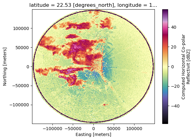
Plot simple PPI#
Now, let’s create our PPI plot! We just use the newly created 2D-coordinates x and y to create a meshplot.
radar["sweep_0"]["DBZ"].plot(x="x", y="y", cmap="ChaseSpectral")
<matplotlib.collections.QuadMesh at 0x79769c2e8d70>
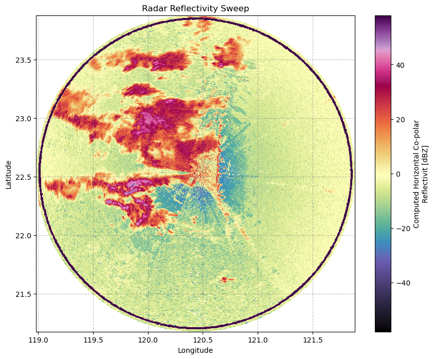
Plot PPI with geographic coordinates#
fig, ax = plt.subplots(figsize=(10, 8))
radar = xd.georeference.get_x_y_z_tree(radar, target_crs=4326)
sweep = radar["sweep_0"]
sweep["DBZ"].plot(x="x", y="y", cmap="ChaseSpectral")
ax.grid(True, which="both", linestyle="--", color="gray", alpha=0.5)
ax.set_xlabel("Longitude")
ax.set_ylabel("Latitude")
ax.set_title("Radar Reflectivity Sweep")
Text(0.5, 1.0, 'Radar Reflectivity Sweep')
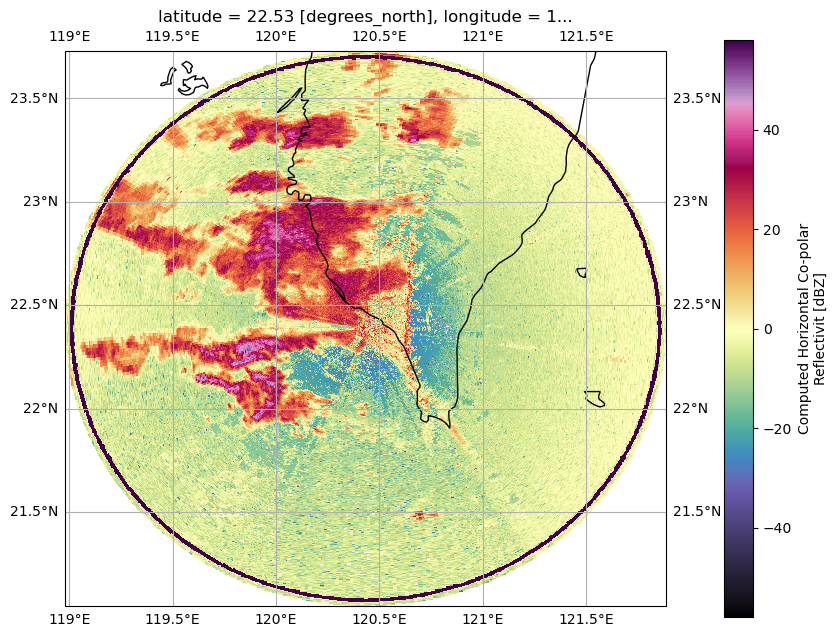
Plot PPI on map with cartopy#
If you have cartopy installed, you can easily plot on maps. We first have to extract the CRS from the dataset and to wrap it in a cartopy.crs.Projection.
proj_crs = xd.georeference.get_crs(radar["sweep_0"].to_dataset(inherit="all_coords"))
cart_crs = cartopy.crs.Projection(proj_crs)
Second, we create a matplotlib GeoAxes and a nice map.
fig = plt.figure(figsize=(10, 10))
ax = fig.add_subplot(111, projection=cartopy.crs.PlateCarree())
radar["sweep_0"]["DBZ"].plot(
    x="x",
    y="y",
    cmap="ChaseSpectral",
    transform=cart_crs,
    cbar_kwargs=dict(pad=0.075, shrink=0.75),
)
ax.coastlines()
ax.gridlines(draw_labels=True)
/home/docs/checkouts/readthedocs.org/user_builds/xradar/conda/latest/lib/python3.13/site-packages/cartopy/mpl/geoaxes.py:1762: UserWarning: The input coordinates to pcolormesh are interpreted as cell centers, but are not monotonically increasing or decreasing. This may lead to incorrectly calculated cell edges, in which case, please supply explicit cell edges to pcolormesh.
  result = super().pcolormesh(*args, **kwargs)
<cartopy.mpl.gridliner.Gridliner at 0x79769c2eb8c0>